Information Provided & Detection Limits
- Conventional AFM: Max AFM scan range = 100µm by 100µm (xy) by 15µm (z). Typical realistic resolution (accommodating tip contact area and depending on contrast mechanism) is 1to 50 nm (xy) and a few Angstroms in (z). For oscillating signals, tens of pm resolution is practical. Common results: Images, point measurements, roughness calculations, height or property histograms. Original data format: Wavemetrics Igor (.ibw).
- Epi-fluorescence imaging:
- The table below summarizes individual pixel sizes and overall fields of view for common microscope configurations, based on our camera specs of 2048x2048 pixels, 6.5µm by 6.5µm each, 37000:1 dynamic range, 0.006 e-/pixel/s (Water Cooled to -30° C). Max z-ranges are typically limited by objective working distance, scattering, and/or autofluorescence. Common results: Images, image Stacks, intensity histograms, feature tracks. Original data format: Images and stacks (.tif); feature tracking (.xlsx).
- Objective and Camera Details:
- The table below summarizes individual pixel sizes and overall fields of view for common microscope configurations, based on our camera specs of 2048x2048 pixels, 6.5µm by 6.5µm each, 37000:1 dynamic range, 0.006 e-/pixel/s (Water Cooled to -30° C). Max z-ranges are typically limited by objective working distance, scattering, and/or autofluorescence. Common results: Images, image Stacks, intensity histograms, feature tracks. Original data format: Images and stacks (.tif); feature tracking (.xlsx).
| Objective: | 10x | 40x | 60x (oil) | 100x |
| nm/pix | 650 | 163 | 108 | 65 |
| with 1.5x mag | 433 | 108 | 72 | 43 |
| xy range (um) | 1331 | 333 | 222 | 133 |
| with 1.5x mag | 887 | 222 | 148 | 89 |
| Hamamatsu Flash4v3: | pix/side: | 2048 | um/pix: | 6.5 |
-
- The tables below summarize excitation and emission wavelengths for which the system is typically configured. Other options can possibly be accommodated for users who can supply the appropriate filters.
- Microscope Filter Wheel:
- The tables below summarize excitation and emission wavelengths for which the system is typically configured. Other options can possibly be accommodated for users who can supply the appropriate filters.
| filter wheel label | Excitation Bandwidth (nm) | Emission Bandwidth (nm) | Part # (real, or cloesest available in 2024) |
| UV | 340-380 (UV) | 435-485 (indigo+blue) | Nikon 96310 UV-2E/C C63936 |
| B | 465-495 (blue) | 515-555 (green) | Nikon B-2E/C, 96311, C65357 |
| G | 528-553 (green) | 590-650 (orange) | Nikon G-2E/C, 96312, C65358 |
| arrows (actually dual: B/G) | CFP, or GFP/YFP: 432-440, 488-510 | 453-480, 525-566 (blue/green) | Chroma 52017 CFP/YFP |
| Bright Field | full spectrum | >420 (UV filtered) | Chroma: 33002, BFT FLD, C53823 |
| G/R | Dual: 458-499, 570-600 (blue/yellow) | 507-541, 610-648 (green/red) | Semrock FITC/Txed-2x-a-nte. EXCITE: FF01-479/585-25, EMIT: FF01-524/628-25 |
-
-
- DG-4 (Hg Arc Lamp and 4 automated filter sets):
-
| Improvision label | TxRed | GFP | Open | CFP |
| low edge (nm) | 576 | 475 | UV | 430 |
| high edge (nm) | 596 | 495 | near IR | 440 |
| filtered color | yellow | blue | full spectrum (Hg arc lamp) | purple |
| Note1: YFP (490-510 nm excitation) may be swappable into 1 of the 4 slots on request. | ||||
| Note2: a manual mirror can be flipped for white light (phosphor LED) excitation instead. | ||||
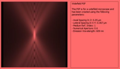
- Deconvolution:
- We use Perkin Elmer’s Improvision Volocity software package to perform deconvolution with z-stacks when applicable. An example of the widefield psf for our 40x air objective at 609nm is shown below.